As I begin my dive into Digital Signal Processing (DSP) for audio applications, I thought it would be good to share what I am learning along the way. A few years ago I sought resources to learn DSP from a professor of mine. He recommended that I check out the book 'Designing Audio Effect Plugins in C++ with DSP Theory' (2013) by Will C. Pirkle. That started a long journey to where I am now, some years later, reviewing and learning from the newest version of the book released in 2019 (ISBN: 978-1-138-59189-9).

This blog post is completely for academic purposes. The book is amazing and I highly recommend it for those looking to get into the world of audio effects plug-ins and digital (audio) signal processing. In these blog posts I will be sharing my notes from the book. My notes are recaps of the book and do not go over the detail with which the book goes over these topics. If you're starting out or would like a more in-depth introduction to these topics, there is no better resource than the source itself.
Amazon: https://www.amazon.com/Designing-Audio-Effect-Plugins-C-dp-1138591939/dp/1138591939

** This article was posted on my former Ghost Blog in 2022.

1 Fundamentals of Audio Signal Processing

In this section we will examine how digital systems handle the acquisition of data, audio reconstruction, and numerical representation of the audio signal.

 1.1 Acquisition of Audio Samples

Incoming analog audio signal is sampled with an analog-to-digital converter (ADC or A/D). ADCs convert an analog signal into a digital signal by taking samples of the analog signal's value at regular intervals.

• How Regular Should We Sample?

"The sampling theorem states that a continuous analog signal can be sampled into discrete data points and then reconstructed into the original analog signal without any loss of information—including inter-sample fluctuations—if and only if the input signal has been band-limited so that it contains no frequencies higher than half the sample rate, also known as the Nyquist frequency or Nyquist rate.  Band-limiting the input signal prior to sampling is known as adhering to the Nyquist criteria." (pg. 3)

Violating the Nyquist frequency will result in an erroneously encoded signal in which the frequencies higher than the Nyquist frequency will "fold back into the spectrum" causing a defect referred to as aliasing.

1.2 Reconstruction of the Audio Signal

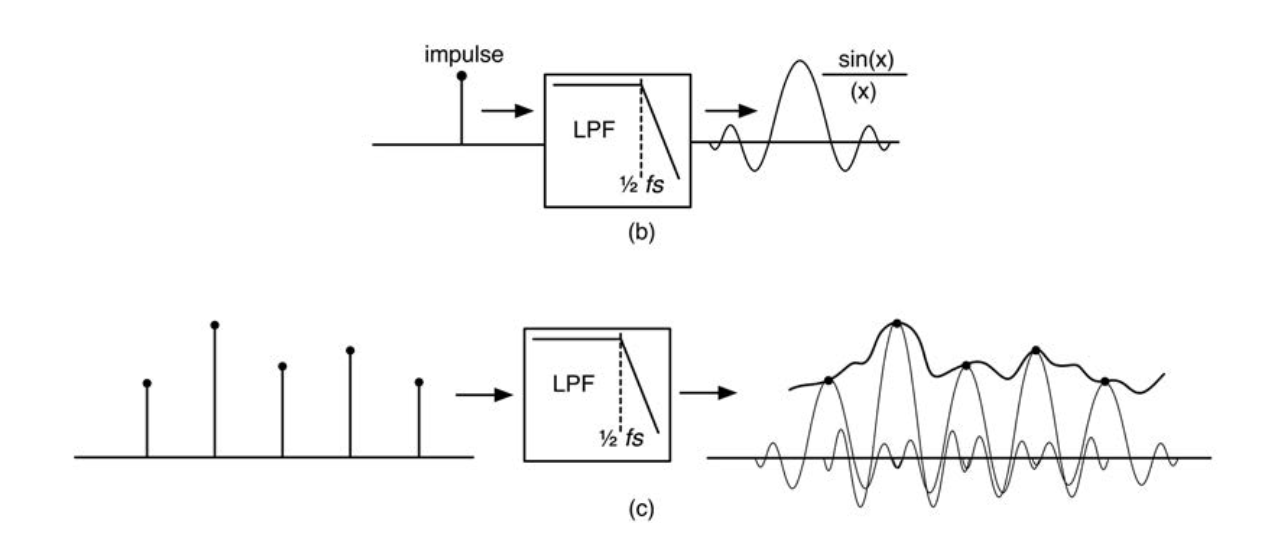
The goal of the digital to analog converter (DAC or D/A) is to take the sampled data points and convert them into analog (continuous) versions of those impulses. This is accomplished by sending the data points through an output filter, called the reconstruction filter. The reconstruction filter uses the sinc( ) function,
 

sinc(x) = sin(x)/x

to recreate the inter-sample fluctuations. When a series of impulses is sent through this function, the resulting set of sin(x)/x pulses overlap with each other and their responses add up linearly. The addition of all the smaller curves and damped oscillations reconstructs the inter-sample curves and fluctuations.

1.3 Signal Processing Systems

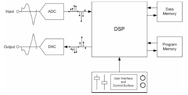
Signal processing systems combine data acquisition devices with microprocessors to run mathematical algorithms on the audio data. A DSP chip is a highly specialized processor designed mainly to run DSP algorithms. DSP devices (or just “DSPs”) feature a core processor designed to multiply and accumulate data because this operation is fundamental to DSP algorithms. Because this process is repeated over and over, modern DSPs use pipelining to fetch the next data while simultaneously processing the current data. A typical signal processing system consists of the following components

1.4 Synchronization and Interrupts

There are two fundamental modes of operation when dealing with incoming and outgoing audio data: synchronous and asynchronous. In synchronous operation, all audio input and output data words are synchronized to the same clock as the DSP.

"An asynchronous system will almost always be interrupt-based. In an interrupt-based design, the processor enters a wait-loop until a processor interrupt is toggled. The processor interrupt is just like a doorbell. When another device such as the A/D has data ready to deliver, it places the data in a predesignated buffer, and then it rings the doorbell by toggling an interrupt pin. The processor services the interrupt with a function that picks up the data, and then goes on with its processing code. The function is known as an interrupt-service routine or an interrupt handler." (2013, pg. 25)

Another source of interrupts is the UI. Each time the user changes a control, clicks a button, or turns a knob, the updated UI control information needs to be sent to the DSP so it can alter its processing to accommodate the new settings.

1.5 Signal Processing Flow

Whether the processing is taking place on a DSP chip or in a plug-in, the overall processing flow, also known as the signal processing loop, remains basically the same.

• A one-time initialization function to set up the initial state of the processor and prepare for the arrival of data interrupts
• An infinite wait-loop, which does nothing but wait for an interrupt to occur
• An interrupt handler which decodes the interrupt and decides how to process—or ignore—the

doorbell

• Data reading and writing functions for both control and data information
• A processing function to manipulate and create the audio output
• A function to set up the variables for the next time around through the loop, altering variables if the

UI control changes warrant it

1.6 Numerical Representation of Audio Data

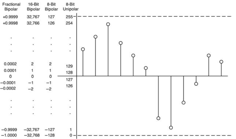
Basic digital audio theory reveals that the number of quantization levels available for coding is q = 2N where N is the bit depth of the signal. Thus an 8-bit system can encode 2ˆ8  values or 256 quantization levels.

• Unipolar (unsigned)

Unipolar data points range of zero to +max, or −min to zero and only has one polarity (+ or −) of data, plus the number zero.

• Bipolar (signed)

Bipolar data points range from −min to +max and is the most common form today; it also includes the number zero.

• Integer

Integer data points are represented with integers and no decimal place.

• Fractional

Fractional data are encoded with an integer and fractional portion, combined as int.frac. Within the fractional data subset are fixed and floating point types.

• Fixed point data fixes the number of significant digits on each side of the decimal point. For example, “8.16” data would have eight significant digits before the decimal place and 16 afterwards.
• Floating point data has a moving mantissa and exponent component. The positive and negative portions are encoded in 2’s complement so that addition of exactly opposite values (e.g. −0.5 and + 0.5) always results in zero.
   

 Converting an integer value to a fractional value is easy:

 Where N = bit-depth of the system.

1.7 Analytical DSP Test Signals

In this section we will cover several fundamental digital signals which will lay the foundation for the DSP theory to come.

The basic signal set consists of the following:

• Direct Current (DC) and Step (0 Hz) (also known as the Heaviside function in Calculus)
• Nyquist
• 1⁄2 Nyquist
• 1⁄4 Nyquist
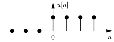
• Impulse (also known as the delta function in Calculus)

These signals serve as an analytical foundation for determining the frequency response of some basic DSP filters.

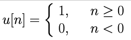
Direct Current (DC) and Step (0 Hz)

The Step function, or Heaviside function, is defined as follows:
 

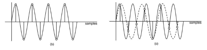
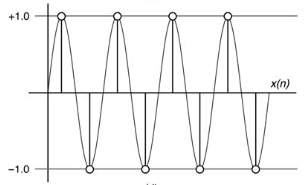
Nyquist

The Nyquist input sequence represents the Nyquist frequency of the system and is independent of the actual sample rate. The Nyquist sequence is {. . . −1, +1, −1, +1, −1, +1, −1, +1 . . .}. The Nyquist sequence represents the highest frequency that can be represented. Any signal above this frequency would alias.

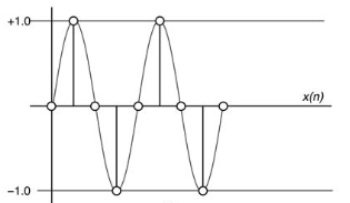
1⁄2 Nyquist

The 1⁄2 Nyquist sequence is { . . . −1, 0, +1, 0, −1, 0, +1, 0, −1, 0, +1, 0, −1, 0, +1, 0 . . .}
 

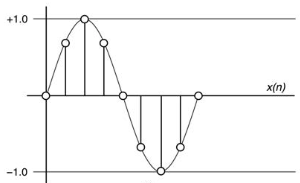
1⁄4 Nyquist

The 1⁄4 Nyquist sequence is {. . . 0.0, 0.707, +1.0, 0.707, 0.0, −0.707, −1.0, −0.707, 0.0 . . .}.

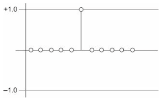
Impulse or Delta Function

The impulse, or Delta, Function contains a single sample with the value 1.0 in an infinitely long stream of zeros. The impulse response of a DSP algorithm is the output of the algorithm after applying the impulse input.

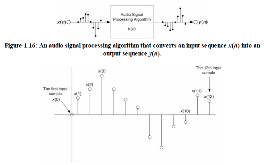
1.8 Signal Processing Algorithms

In the specialized case of audio signal processing, an algorithm is a set of instructions that operates on data to produce an audio output bit-stream.

Conventions and rules:

• x(n) is always the input sequence; the variable n represents the location of the nth sample of the x- sequence.
• y(n) is always the output sequence; the variable n represents the location of the nth sample of the y- sequence.
• h(n) is the impulse response of the algorithm; a special sequence that represents the algorithm output for a single sample input or impulse.
• For real-time processing, the algorithm must accept a new input sample (or set of samples), do the processing, then have the output sample(s) available before the next input arrives; if the processing takes too long, clicks, pops, glitches, and noise will be the real-time result.

1.9 Book Keeping

DSP algorithms use the position of the current sample and make everything relevant to that sample. On the next sample period, everything gets reorganized in relation to the current sample again. This is the method used for defining the I/O characteristics of the algorithm, called the transfer function.

 Bookkeeping Rules:

• The current sample is labeled “n.”
• Previous samples are negative, so x(n − 1) would be the previous input sample.
• Future samples are positive, so x(n + 1) would be the next input sample relative to the current one.
• On the next sample interval, everything is shuffled and referenced to the new current sample, x(n).

1.10 The One-Sample Delay

Whereas analog processing circuits like tone controls use capacitors and inductors to alter the phase and delay of the analog signal, digital algorithms use time delay instead.

"In our algorithm diagrams, a delay is represented by a box with the letter z inside. The z-term will have an exponent such as z−5 or z+2 or z0; the exponent codes the delay in samples following the same bookkeeping rules, with negative (−) exponents representing a delay in time backwards (past samples) and positive (+) representing delay in forward time (future samples). We call z the delay operator and as it turns out, it will be treated as a mathematical operation." (2019, pg. 11)

Delay Rules:

• Each time a sample goes into the delay register (memory location), the previously stored sample is ejected.
• The ejected sample can be used for processing or deleted.
• The delay elements can be cascaded together with the output of one feeding the input of the next to create more delay time.

1.11 Multiplication With a Scalar

It is a sample-by-sample operator that simply multiplies the input samples by a coefficient.

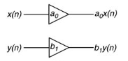
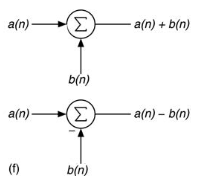
1.12 Addition and Subtraction

The operation of mixing signals is really the mathematical operation of addition.

1.13 Difference Equations

By convention, the output sequence of a DSP algorithm is named y(n) and the mathematical equation that relates it to the input is called the difference equation. The difference equation does not necessarily require a subtraction (difference) operation. Its name corresponds to the analog equivalent version called the differential equation.

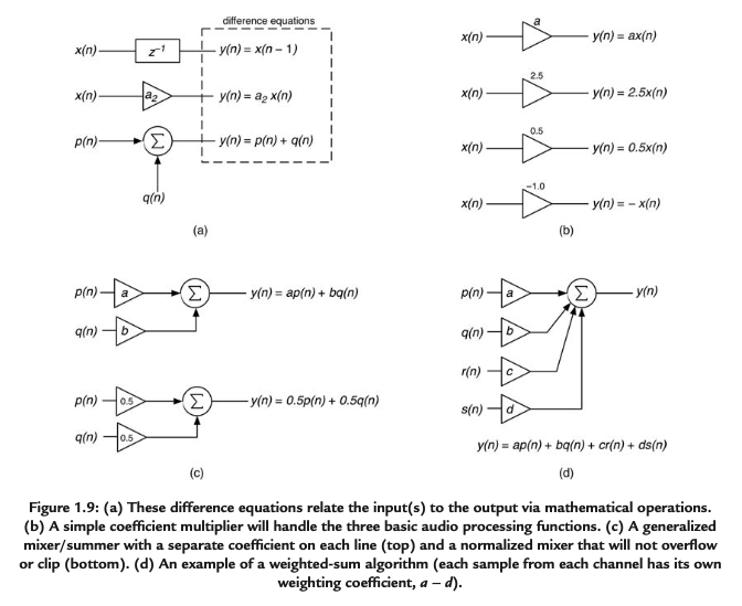
1.14 Gain, Attenuation, and Phase Inversion

Each of these fundamental audio processing functions are the result of multiplication by a scalar. Gain is produced when a signal is multiplied by a coefficient greater than one. Attenuation is produced when a signal is multiplied by a coefficient between 1 and 0. Attenuation is produced when a signal is multiplied by a negative coefficient.

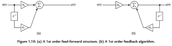
1.15 First Order Feed-Forward and Feedback Algorithms

For a feed-forward structure, the input is split into current input x(n) and delayed input x(n − 1) signal paths. Each path

is weighted with a coefficient a0 and a1; the current output y(n) is the simple sum of these two paths.
In the feedback version the current input feed-forward branch scaled with a0 and a feedback path that recycles the output y(n) after delaying it by one sample to form y(n − 1); this delayed output path is scaled with −b1 and summed with the input path.